
Introduction
Set up
We are given the dataset \(X = \{ (\mathbf{x}_n, \mathbf{y}_n) \mid n=1,..,N \}\) that is a sequence of data points \((\mathbf{x}_n, \mathbf{y}_n) \in \mathbb{R}^{d_x} \times \mathbb{R}^{d_y}\), where \(N\) is the number of data points. \(\mathbf{x_n}\) are sampled from an unknown distribution \(\mathcal{D}\), and mapped to \(\mathbb{R}^{d_y}\) with an unknown function \(f(\mathbf{x_n}) = \mathbf{y_n}\), \(f\) determines the correct \(\mathbf{y}\) for each \(\mathbf{x}\).
Neural network
The neural nework is a parametric function \(NN: \mathbb{R}^{d_x} \to \mathbb{R}^{d_y}\) that tries to approximate the unknown \(f\): \[\hat{\mathbf{y}} = NN(\mathbf{x}, \Theta).\] \(\Theta\) is a vector of parameters. The neural network is composed of \(K\) layers (indexed with \(l=1,..,K\)) of simple functions \(g_l\) (neurons) whereby the output of a layer \(l\), \(\mathbf{o}_l\), plays the role of an input for the next layer \(l+1\). \(\Theta\) lumps together parameters of all layers (\(\mathbf{w}^l\) for all \(l\)).

\[\mathbf{o}^l = g_l(\mathbf{a}^l) = g_l(\mathbf{w}^l\mathbf{o}^{l-1})\] \[\mathbf{a}^l = \mathbf{w}^l\mathbf{o}^{l-1} = \mathbf{w}^lg_l(\mathbf{a}^{l-1})\]
where \(g_l\) is a nonlinear function, \(\mathbf{w}^l\) is \(N_l \times (N_{l-1}+1)\) matrix of parameters for the layer \(l\), \(N_l\) is the number of neurons in layer \(l\), \(\mathbf{o}^{l-1}\) is a \((N_{l-1}+1)\) column vector, \(\mathbf{a}^{l}\) is a \(N_{l}\) column vector. \(l=1,...,K\) is an index of the layer, \(K\) is the number of layers. The output of layer 0, corresponds to the input given to network, whereas the output of last K-th layer gives the output of the network: \(\hat{\mathbf{y}}_n \equiv \mathbf{o}^K\), \(\mathbf{o}^0 \equiv \mathbf{x}_n\).
Component-wise: \[a_i^l = \sum_{j=0}^{N_{l-1}} w_{ij}^l o_j^{l-1} = \sum_{j=1}^{N_{l-1}}w_{ij}^l o_j^{l-1} + b_i^l\]
where \(a_i^l\) is the activation of \(i\)-th neuron in layer \(l\), \(o_j^l\) is the output of \(j\)-th neuron, \(b_i^l = w_{i0}^l\) is bias (\(o_0^{l-1} \equiv 1\)), \(\Theta = \{ w_{ij}^l\ \mid \ \text{for all }i,j,l \}\).
We need to measure how bad is the approximation of \(f\) given by \(NN\). For this, we define the loss function \(L^{\text{true}}(\Theta)\): \[L^{\text{true}}(\Theta) = E_{\mathbf{x} \sim \mathcal{D}}[C(\hat{\mathbf{y}}(\mathbf{x}), f(\mathbf{x}))]\]
Ideally, the parameters of the network (\(\Theta\)) are chosen so that the loss is minimized:
\[\Theta^{*} = \mathrm{argmin}_{\Theta} L^{\text{true}}(\Theta)\]
Here \(C\) is the cost function that measures how bad \(NN\) performs for one point, e.g. \(C(\mathbf{z}, \mathbf{y})=\|\mathbf{z}-\mathbf{y}\|_2^2\).
In practice, having finite data set \(X\), we approximate expectation with average:
\[L^{\text{real}}(\Theta) \approx L(X, \Theta) = \frac{1}{N}\sum_{n=1}^{N}C(\hat{\mathbf{y}}(\mathbf{x}_n),\mathbf{y}_n)\]
To evaluate if this approximation was reasonable, we compute empirical loss \(L(X_{\text{test}}, \Theta)\) on another data set \(X_{\text{test}}\) and make sure that it is not too large compared to \(L(X, \Theta)\).
Searching for a good network
To minimize \(L\), gradient descent can be used, that is \(\Theta\) is updated according to:
\[\Theta_{t+1} = \Theta_t - \eta \nabla L(X, \Theta_t)\] Here \(t\) iteration of the algorithm, \(\eta\) is learning rate, \(\nabla\) denotes gradient operator.
The computation of the gradient is often done with a numerical version of automatic differentiation so-called backpropagation (it has nothing to do with backpropagation of action potential in Neuroscience).
Let’s derive components of \(\nabla L(X, \Theta_t)\) for a layer \(l\).
\[\frac{\partial L}{\partial w_{ij}^l} = \frac{1}{N} \sum_{n=1}^{N} \frac{\partial C(\hat{\mathbf{y}}(\mathbf{x}_n),\mathbf{y}_n)}{\partial w_{ij}^{l}}\] Or in vectorized form:
\[\mathbf{J}_L^l = \frac{1}{N}\sum_{n=1}^N \mathbf{J}_C^l(\hat{\mathbf{y}}(\mathbf{x}_n),\mathbf{y}_n)\]
Cost function \(C\) depends on \(\hat{\mathbf{y}}\), whereas each \(\hat{\mathbf{y}}\) (or output of the last layer) depends on outputs of previous layers \(\mathbf{o}^{l'}\) \(l`<K\), whereas parameters corresponding to layer \(l\) first appear in \(\mathbf{o}^l\):
\(C = C\left(\hat{\mathbf{y}}\left(\mathbf{o}^K(\mathbf{o}^l), \mathbf{o}^{K-1}(\mathbf{o}^l),...,\mathbf{o}^l\right)\right)\) and \(\mathbf{o}^l = \mathbf{o}^l(\mathbf{w}^l)\).
We can thus write:
\[\frac{\partial C}{\partial w_{ij}^l} = \frac{\partial C}{\partial a_i^l} \frac{\partial a_i^l}{\partial w_{ij}^l} = \frac{\partial C}{\partial o_i^l} \frac{\partial o_i^l}{\partial a_i^l} \frac{\partial a_i^l}{\partial w_{ij}^l} = \frac{\partial C}{\partial o_i^l} g_l'(a_i^l) o_j^{l-1} = \delta_i^l o_j^{l-1} \]
We can define Jacobian for \(C\) for each layer (\(J_{ij}^l = \frac{\partial C}{\partial w_{ij}^l}\)) and rewrite this equation in vectorized form:
\[\mathbf{J}^l = (\mathbf{\delta}^l) (\mathbf{o}^{l-1})^T\]
Here \(\delta_i^l = \frac{\partial C}{\partial a_i^l}\). In this formula, we can easily compute all except \(\frac{\partial C}{\partial o_i^l}\). However, for the last layer \(l=K\), as \(o_i^K = \hat{y}_i\), we can compute: \[\frac{\partial C}{\partial w_{ij}^K} = \frac{\partial C(\hat{\mathbf{y}}(\mathbf{x}),\mathbf{y})}{\partial \hat{y}_i} g_K'(a_i^K) o_j^{K-1},\]
which in vectorized form would be:
\[\mathbf{J}^K = (\nabla_{\hat{y}}C \odot g_K'(\mathbf{a}^K)) (\mathbf{o}^{K-1})^T.\]
If we know \(\frac{\partial C}{\partial o_i^l}\) and we can express \(\frac{\partial C}{\partial o_j^{l-1}}\) as a function of \(\frac{\partial C}{\partial o_i^l}\). After this, we will be able to compute \(\frac{\partial C}{\partial w_{ij}^{l-1}}\). As we already know \(\frac{\partial C}{\partial w_{ij}^{l}} = \frac{\partial C(\hat{\mathbf{y}}(\mathbf{x}_n),\mathbf{y}_n)}{\partial \hat{y}_i}\), we can recursively compute all components of \(\nabla_{\Theta} C\) going backwards in layers.
Let’s find \(\frac{\partial C}{\partial o_{j}^{l-1}} \mapsto \frac{\partial C}{\partial o_{i}^{l}}\).
\[C = C(\mathbf{o}^l(\mathbf{o}^{l-1}))\]
\[\frac{\partial C}{\partial o_{j}^{l-1}} = \sum_{i=0}^{N_l} \frac{\partial C}{\partial o_{i}^{l}} \frac{\partial o_i^{l}}{\partial o_{j}^{l-1}} = \sum_{i=0}^{N_l} \frac{\partial C}{\partial o_{i}^{l}} g_l'(a_i^l) w_{ij}^l = \sum_{i=0}^{N_l} \delta_i^l w_{ij}^l\]
We can rewrite in terms of \(\delta_i^l\):
\[\delta_j^{l-1} = \frac{\partial C}{\partial o_{j}^{l-1}} g_{l-1}'(a_j^{l-1}) = \left(\sum_{i=0}^{N_l} \delta_i^l w_{ij}^l\right) g_{l-1}'(a_j^{l-1})\]
In vectorized form:
\[\mathbf{\delta}^{l-1} = \left( (\mathbf{w}^l)^T \mathbf{\delta}^l \right) \odot g_{l-1}'(\mathbf{a}^{l-1})\]
Here \(\odot\) is elementwise product.
Algorithm
Forward pass for \((\mathbf{x}, \mathbf{y}) \in X\) to compute activations and outputs:
- Set \(\mathbf{o}^0 = \mathbf{x}\)
- For \(l=1,...,K\):
- \(\mathbf{a}^l = \mathbf{w}^l\mathbf{o}^{l-1}\)
- \(\mathbf{o}^l = g_l(\mathbf{a}^{l})\)
Backpropagation to compute gradient of the loss function:
- Take \(A \subseteq X\)
- For each \((\mathbf{x}_n, \mathbf{y}_n) \in A\):
- do forward pass to compute all \(g_l(\mathbf{a}^l)\)
- compute \(\mathbf{\delta^K} = \nabla_{\hat{y}}C \odot g_K'(\mathbf{a}^K)\)
- compute \(\mathbf{J}^K = (\mathbf{\delta}^K) (\mathbf{o}^{K-1})^T\)
- For \(l=K,K-1,...,2\)
- \(\mathbf{\delta}^{l-1} = \left( (\mathbf{w}^l)^T \mathbf{\delta}^l \right) \odot g_{l-1}'(\mathbf{a}^{l-1})\)
- compute \(\mathbf{J}^{l-1} = (\mathbf{\delta}^{l-1}) (\mathbf{o}^{l-2})^T\)
- Compute \(\mathbf{J}_L^l = \frac{1}{|A|}\sum_{n=1}^{|A|} \mathbf{J}_C^l(\hat{\mathbf{y}}(\mathbf{x}_n),\mathbf{y}_n)\) for all \(l\)
Stochastic gradient descent:
- For \(t=1,...,T\) do
- Select randomly \(A \subset X\)
- Do backpropagation for \(A\) to compute gradient \(\mathbf{J}_L^l\)
- For each \(l=1,...,K\) do
- \(\mathbf{w}^l_t = \mathbf{w}^l_{t-1} - \eta \mathbf{J}_L^l\)
Getting hands dirty with python and NumPy
First, I defined some useful general functions.
```python
import numpy as np
from copy import deepcopy
from functools import partial
import matplotlib.pyplot as plt


def sigmoid(x, derivative=False):
    s = 1.0 / (1.0 + np.exp(-x))
    if derivative:
        return s * (1.0 - s)
    else:
        return s
sigmoid.name = 'sigmoid'


def updated(d, dupdate):
    d = deepcopy(d)
    d.update(dupdate)
    return d

def shuffled(x):
    x = deepcopy(x)
    np.random.shuffle(x)
    return x


def dataToBatches(data, batch_size):
    lenData = len(data)
    ilast = lenData // batch_size
    start = 0
    while start < lenData-1:
        stop = min(lenData, start + batch_size)
        yield data[start:stop]
        start += batch_size


def grad_l2_cost(y, target):
    return (target-y)

def l2_cost(nn, datapoint):
    image, label_one_hot = datapoint
    return np.mean((nn.forward(image)-label_one_hot)**2)

def lossData(nn, data):
    return np.mean(list(map(partial(l2_cost, nn), data)))

def accuracy(nn, data):
    return np.mean(
        [ np.argmax(nn.forward(d[0])) == np.argmax(d[1])
          for d in data
        ])

def one_hot_mnist(label):
    x = np.zeros(10)
    x[label] = 1.0
    return x
```
Let’s define neural network class.
```python
class Layer():
    def __init__(self, parameters):
        self.W = parameters['init_weights'](
                parameters['n_out'],
                parameters['n_in'])
        self.b = parameters['init_biases'](
                parameters['n_out'])
        self.Wb = np.hstack([self.b[:, np.newaxis], self.W])
        self.act_func = parameters['act_func']
        self.dact_func = parameters['dact_func']
        self.dactivation = None # to keep track of its activation
        self.output = None
    def forward(self, inp):
        inp = np.insert(inp, 0, 1.0)
        activation = np.matmul(self.Wb, inp)
        self.dactivation = self.dact_func(activation)
        output = self.act_func(activation)
        self.output = np.insert(output, 0, 1)
        return output
    def setLast(self):
        for attr in ['output']:
            setattr(self,
                    attr,
                    getattr(self, attr)[:-1])

    def __repr__(self):
        return "(Input, Output) size: {}".format(self.W.shape[::-1]) + "\n" +\
               "Activation: {}".format(self.act_func.name) + "\n"

class Network():
    def __init__(self, layers_pars, grad_cost):
        self.layers = [Layer(par) for par in layers_pars]
        self.grad_cost = grad_cost
    def forward(self, inp):
        out = inp
        for l in self.layers:
            out = l.forward(out)
        l.setLast()
        return out
    def __repr__(self):
        desc = ''
        for i, l in enumerate(self.layers):
            desc += "Layer {}\n".format(i)
            desc += repr(l) + "\n"
        return desc
    def describe(self):
        print(repr(self))

    def gradient(self, data):
        sum_Jls = np.zeros(len(self.layers))
        lenData = 0
        for x, y in data:
            lenData += 1
            output = self.forward(x)

            delta = self.grad_cost(y, output)\
                    * self.layers[-1].dactivation
            delta = delta[:, np.newaxis]

            Jl  = np.matmul(delta,
                            self.layers[-2].output[np.newaxis, :])
            Jls = [Jl]

            for l in range(len(self.layers)-1, 0, -1):

                q1 = np.matmul(self.layers[l].Wb.T, delta)
                q2 = self.layers[l-1].dactivation[:, np.newaxis]
                delta = q1[1:] * q2

                outprev = \
                        self.layers[l-2].output[np.newaxis, :]\
                        if l-2 > -1 else\
                        np.insert(x, 0, 1)[np.newaxis]
                Jl  = np.matmul(delta, outprev)
                Jls.append(Jl)
            sum_Jls = [ old+Jl for old,Jl in zip(sum_Jls, Jls) ]
        mean_Jls = [ old / lenData for old in sum_Jls ]
        # correct for reversion as a result of backward computation
        mean_Jls = mean_Jls[::-1]
        return mean_Jls

    def SGD(self, data,
            batch_size=100,
            max_iter=None,
            learning_rate=0.01):
        if max_iter is None:
            max_iter = len(data)
        dataS = shuffled(data)
        for i, batch in enumerate(
                dataToBatches(dataS,
                              batch_size=batch_size)):
            if i > max_iter:
                break
            Jls = self.gradient(batch)
            for l in range(len(self.layers)):
                self.layers[l].Wb -= learning_rate * Jls[l]
```
Let’s make a simple network where \(g_l(x) = 1/(1+e^{-x})\) is the same for all layers, load MNIST data and train network to classify digits.
```python
def mkSimpleNetwork(ns_per_layer):
        parameters =\
            { 'init_weights': np.random.randn
            , 'init_biases' : np.random.randn
            , 'act_func'    : sigmoid
            , 'dact_func'   : partial(sigmoid, derivative=True)
            }
        layers_pars = []
        for n_in, n_out in zip(ns_per_layer[:-1],
                               ns_per_layer[1:]):
            layers_pars.append(
                updated(parameters,
                        { 'n_in'  : n_in
                        , 'n_out' : n_out
                        }))
        return Network(layers_pars, grad_l2_cost)


def getData(
        mnist_tuple,
        subset=30000,
        shuffle=True
        ):
    images, labels = mnist_tuple
    # Sequence X
    data = list(
            zip(images,
                list(map(one_hot_mnist, labels))))
    if shuffle:
        data = shuffled(data)
    if subset:
        data = data[:subset]
    return data


def scaleData(data, scaler=lambda x: np.array(x)/255.0):
    return [(scaler(img), lbl) for img, lbl in data]

# helpers that are needed later on (skip them for now).

def extend_Wbls(nn, Wbls):
    for i, l in enumerate(nn.layers):
        Wbls[i] = np.vstack([Wbls[i], l.Wb.flatten()])

def plot_save(nn, loss, accs, Wbls, fpath='nnTrain.png'):
    fig, axs = plt.subplots(
            2+len(nn.layers), 1,
            figsize=(6, 6))
    for k in loss.keys():
        axs[0].semilogy(loss[k], label=k)
        axs[1].plot(accs[k], label=k)
    axs[0].set_ylabel('loss')
    axs[0].legend()
    axs[1].set_ylabel('accuracy')
    axs[1].legend()
    for i in range(len(nn.layers)):
        ax = axs[2+i]
        c = ax.pcolor(Wbls[i].T, cmap='RdBu_r')
        ax.set_ylabel("$\mathbf{w}^%i$" % (i+1))
        fig.colorbar(c, ax=ax)
    plt.tight_layout()
    fig.savefig(fpath)
    plt.close()


if __name__ == '__main__':

    # Load and preprocess MNIST data

    from mnist import MNIST
    mndata = MNIST('/home/ilya/Downloads/MNIST/')

    d = {}
    d['train'] = scaleData(getData(
            mndata.load_training()))
    d['test']  = scaleData(getData(
            mndata.load_testing()))

    # Create simple network with two layers

    nn = mkSimpleNetwork([784, 50, 10])

    # initialize measurables

    loss  = {k:[lossData(nn, v)] for k, v in d.items()}
    accs  = {k:[accuracy(nn, v)] for k, v in d.items()}
    Wbls  = [l.Wb.flatten() for l in nn.layers]

    # training loop

    for n_epoch in range(30):
        nn.SGD(d['train'],
               max_iter=None,
               batch_size=8,
               learning_rate=3.0)
        # compute measures and plot results
        for k in d.keys():
            loss[k].append(lossData(nn, d[k]))
            accs[k].append(accuracy(nn, d[k]))
        extend_Wbls(nn, Wbls)
        plot_save(nn, loss, accs, Wbls)
        print("Epoch {}: loss: {} acc: {}".format(
                n_epoch,
                loss['test'][-1],
                accs['test'][-1]))
```
Results
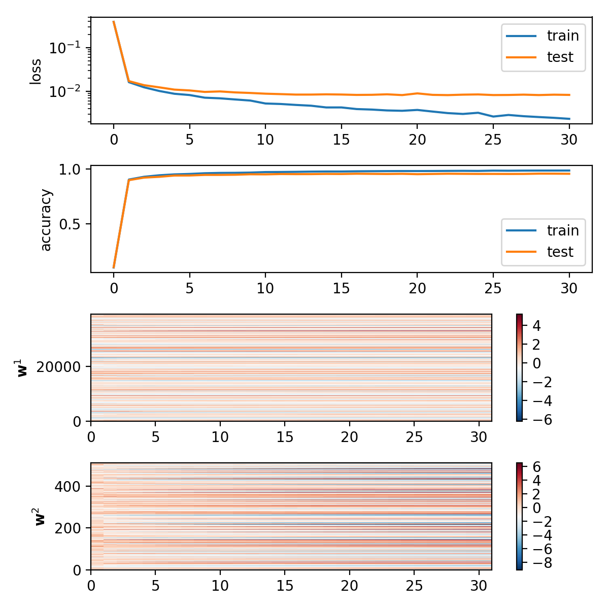
Epoch 0: loss: 0.016991653848590874 acc: 0.8966
Epoch 1: loss: 0.013715554862541645 acc: 0.9196
Epoch 2: loss: 0.012228999662532923 acc: 0.9269
Epoch 3: loss: 0.010847338415188106 acc: 0.9385
Epoch 4: loss: 0.01038737127915931 acc: 0.939
Epoch 5: loss: 0.009598660621545196 acc: 0.9442
Epoch 6: loss: 0.009858286550737687 acc: 0.9443
Epoch 7: loss: 0.009359748620839778 acc: 0.9457
Epoch 8: loss: 0.009088295631916992 acc: 0.95
Epoch 9: loss: 0.008745593652667713 acc: 0.9492
Epoch 10: loss: 0.008550893034509434 acc: 0.9521
Epoch 11: loss: 0.008339602288365305 acc: 0.9513
Epoch 12: loss: 0.00834561132452328 acc: 0.9515
Epoch 13: loss: 0.008456136266077822 acc: 0.9532
Epoch 14: loss: 0.008365949090187232 acc: 0.9525
Epoch 15: loss: 0.008197821605744322 acc: 0.9549
Epoch 16: loss: 0.008246864203031709 acc: 0.9536
Epoch 17: loss: 0.008465551030755258 acc: 0.9525
Epoch 18: loss: 0.008124560552781017 acc: 0.9541
Epoch 19: loss: 0.008889806361243542 acc: 0.9508
Epoch 20: loss: 0.008222358936366456 acc: 0.9528
Epoch 21: loss: 0.008115327748820329 acc: 0.9549
Epoch 22: loss: 0.008307595954575276 acc: 0.9539
Epoch 23: loss: 0.008410497112609237 acc: 0.9531
Epoch 24: loss: 0.008138048542561003 acc: 0.9532
Epoch 25: loss: 0.008175355271420938 acc: 0.9527
Epoch 26: loss: 0.008317691955677251 acc: 0.9531
Epoch 27: loss: 0.008137449156834158 acc: 0.9556
Epoch 28: loss: 0.008301935092177169 acc: 0.9554
Epoch 29: loss: 0.008204441135138874 acc: 0.9545